Subtomogram Averaging (STA) in RELION5

We will now use the particle positions obtained from Template Matching to perform STA on our target of interest (here, cytosolic ribosomes).

In the following section, the parameters you need to use in the RELION Running tab will depend on your system, e.g. if you run on a local machine, or through a computing cluster, etc …

To know whether our job is going to run on GPU or CPU, here’s a list:

• Make pseudo-subtomos (CPU)
• 3D initial model (single GPU)
• 3D classification (GPU normally, but CPU if not doing alignments)
• 3D auto-refine (GPU)
• 3D multi-body (GPU)
• Tomo reconstruct particle (CPU)
• Tomo CTF refinement (CPU)
• Tomo frame alignment (CPU)
• Local resolution (CPU)

Table of Contents

• Extract your particles and check your average
• Refining and cleaning your particles
• Fast alignment using 3D classification with a single class
• 3D classification without alignment
• Creating a mask
• 3D Refinement
• Post-processing
• More classification or going to High-resolution?
• CTF and alignment refinement cycle
• Run CTF refinement
• Run Bayesian polishing
• What to do next?

Extract your particles and check your average

The first step to begin Subtomogram Averaging (STA) is to run an Extract Subtomos job. This job will extract cropped subtomograms from all tilts, around the centre of the particle positions we identified using Template Matching.

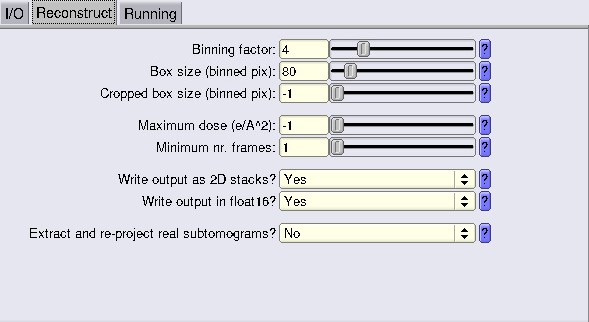
Typically, we start with a binning of 4 or sometimes even 8. We use high binning in the initial steps because the focus is on cleaning and roughly aligning the particles—high-resolution information is not essential at this stage. In this example, we start at bin 4. You want the box size to be larger than your target—ideally at least ~1.5 times larger. Ribosomes are approximately 350 Å wide, which corresponds to about 46 pixels at bin 4.

In general, it’s best to use box sizes that are powers of 2 or 3. These “magic numbers” optimise computational performance. You can find more about that here: https://blake.bcm.edu/emanwiki/EMAN2/BoxSize. In our case, 46 is not ideal, and we want something about 1.5 to 2 times larger anyway. A box size of 72 or 84 pixels would be appropriate, let’s use 84. Of course the larger the box, the longer the computation time.

You want to use the new RELION5 “Write out as 2D stacks” for faster processing. Here for inputs, we used fused particles from Gain1 and Gain2 and created a tomograms.star containing both Gain1 and Gain2 tomos. Fusing particle list can be done in RELION (Join star files) or using the pytom_merge_stars.py from pyTOM. For the concatenated tomograms.star you can just copy/paste the info below the header of Gain1 into the tomograms.star of Gain2 and create a concatenated tomograms_gain1n2.star.

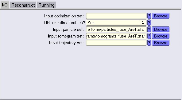
At this stage, you can check how the extracted particles look.

To do this, run a Reconstruct Particle job. In the I/O tab, use the optimisation_set.star file that was generated during the Extract Subtomo job. In the Average section, make sure to set the Box size and Binning factor to exactly the same values you used in the extraction step.

Once the job is complete, you can open the resulting average in Chimera, ChimeraX, or IMOD. The reconstructed volume is typically saved as data_merged.mrc or merged.mrc inside the ~/ReconstructParticleTomo/job00X directory. The result should resemble your expected structure—in this case, a low-resolution ribosome.

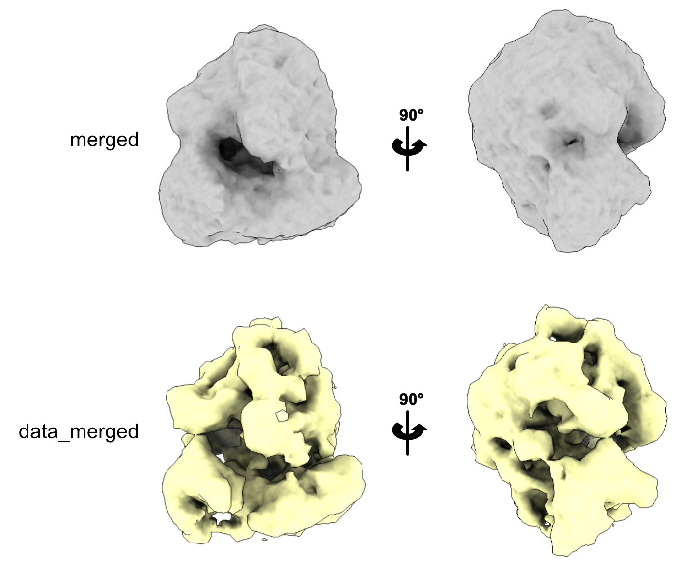
This works well here because we used Template Matching, which provides initial orientation angles. If your particles were picked using a different method, you might need to generate an initial model using the 3D Initial Model job instead.

This initial average will serve as a reference for the next steps, such as 3D classification or refinement.

Refining and cleaning your particles

To improve your average, you have a few key options—mainly alignment and classification. You can perform both simultaneously or run them separately, depending on your goal.

Just like in single-particle analysis, achieving high resolution requires a homogeneous particle set. That’s where classification comes in—it helps you sort out different types of particles or complexes (e.g., ribosomes vs. HSP60), remove junk or noise, and identify structural heterogeneity within a complex (e.g. different translational states of ribosomes).

The first step here is to clean out false positives that may have been picked during Template Matching.

A good approach is to first align all particles together using a quick local refinement. Since our particles already have initial orientations from pytom, a fast alignment with local searches only should be sufficient at this stage.

Once you’ve done that, you can proceed to classification without alignment to separate good particles from bad ones, or to distinguish between different structural states.

Fast alignment using 3D classification with a single class

To align your particles, you have two option, 3D Refinement and 3D Classification. 3D Refinement is the best but is a bit more time consuming, because of how it handles the particle, than 3D classification. At this first step we can use 3D classification, which is a bit less accurate, but faster.

Let’s launch an alignment with the 3D classification using only one class.

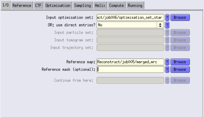
I/O Tab

• Input images STAR file: Use the particles.star file generated by the PseudoSubtomo job.
• Reference map: Use the merged.mrc file produced by the ReconstructParticleTomo job.

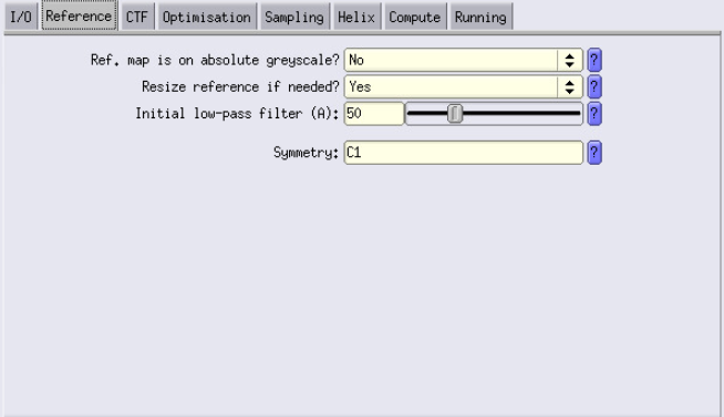
Reference Tab

• Initial low-pass filter: Start with 50 Å. Later, adjust this value to be slightly above the estimated resolution from the previous step. This is important to low-pass filter your reference to avoid over-fitting.
• Example: If 3D Classification gave you a resolution of 22 Å, set this to 25 Å in 3D Refinement.
• Symmetry: We don’t work with a symmetric complex. If you do, I would recommend initially not applying symmetry. Apply it in later stages.

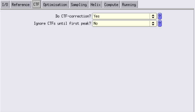
CTF Tab

• CTF Correction: Always enable this.
• Ignore CTFs until first peak: It can be useful to turn on at the beginning, especially for initial alignment and classification. This option acts like a low-pass filter.

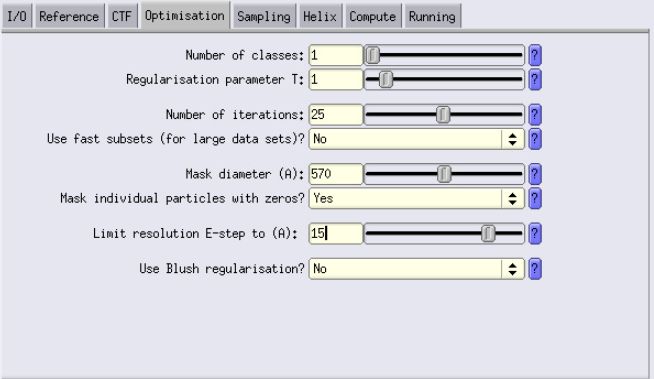
Optimisation Tab

• Number of classes: Set to the number of desired classes. Current case: We are using 1 class.
• T parameter: This is a parameter that you will have to play with. Usually launching multiple jobs with different T values is smart (e.g 0.5, 1, 2 and 4)
• Number of iterations: Start with the default of 25.

• Mask diameter: Should be about 90% of the box size.
  Example: For box size = 84 px, pixel size = 1.91 Å, binning = 4:
  84 × 1.91 × 4 × 0.9 = ~570 Å

• Limit resolution E-step to: To avoid overfitting and noisy reconstructions, set this to the Nyquist resolution at your current binning.
  Example: 1.91 × 4 × 2 = ~15 Å

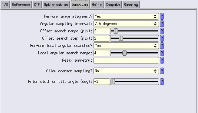
Sampling Tab

• Perform alignment: Set to Yes (since we are aligning). If not aligning, set to No.
• Off search range and step. This defines the translation parameters, how much you let your thing move in the box. Our particles should be centred thanks to TM, and we are high binning, so best is use small values like a range of 2 and a step of 1.
• Local searches only: Enable this, and use the suggested parameters. This overrides the Angular sampling interval. We only want to perform local searches because our particles are already well aligned from TM.

Helix Tab

• Not applicable in our case. Leave it untouched. This is only if you are working with something with helical symmetry, e.g. a filament.

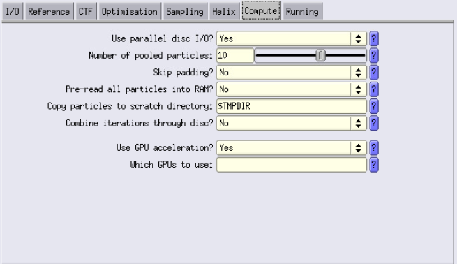
Compute Tab

• Configure settings as shown.
• Enable GPU acceleration only if performing image alignment. If not aligning, disable GPU acceleration.

Adapt the running parameters, and press Run!

When running refinement or classification in RELION, it’s helpful to keep track of progress using a few key metrics in the output files.

You can run these commands from the terminal, in the folder of the job.

• Monitor Resolution Over Iterations This will give you the resolution for each iteration. Ideally, it should improve (i.e., the number decreases) as refinement proceeds.

   grep _rlnCurrentResolution run_it???_model.star
  

• Follow class population and resolution If you’re running classification, use relion_star_printtable to examine how the classes evolve:

   relion_star_printtable run_it001_model.star data_model_classes rlnClassDistribution rlnEstimatedResolution
  

• Monitor Class Convergence (Optimum Changes) Track how well classes are stabilising. This number should start high (near 1) and trend toward 0 as the classes converge

   grep _rlnChangesOptimalClasses run_it???_optimiser.star
  

Let’s see how the resolution evolved over time in that particular case:

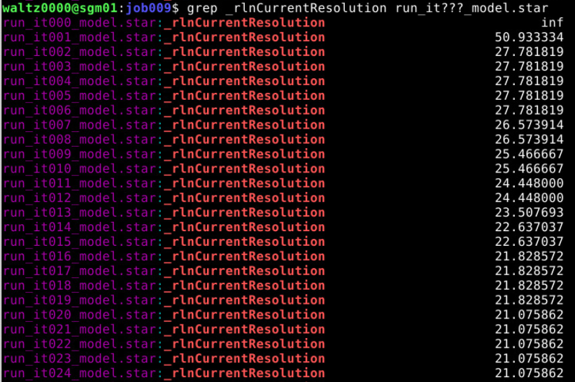
You can see that from iteration 20 it stopped decreasing. This is the iteration that we are going to select to continue.

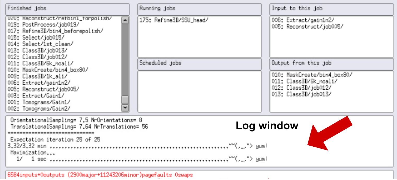
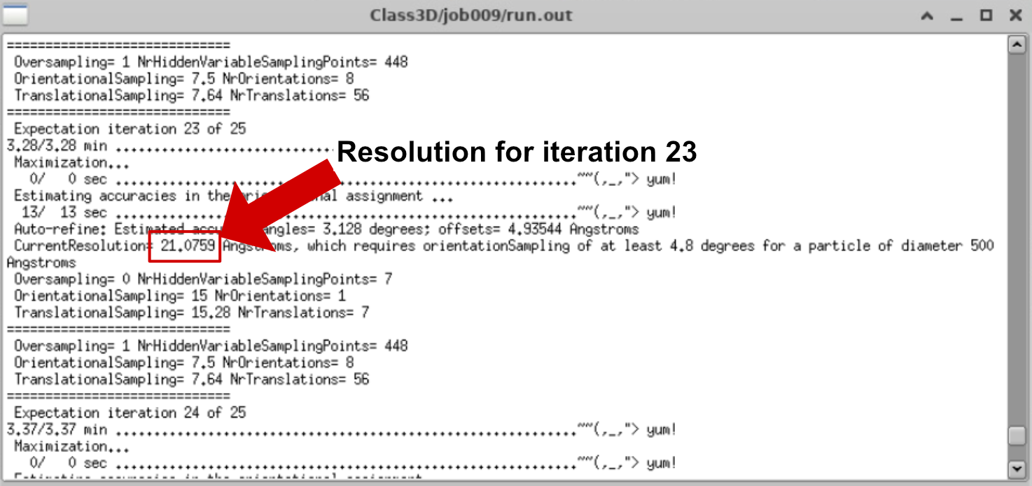
You can also see the resolution at each iteration in the RELION GUI, in the log window. Double click on the log window and it will pop up. You will be able to scroll through the log and check the resolution.

We can also open our volumes in ChimeraX and check if it improved. Remember that this step is almost always mandatory! Even if your resolution is increasing, the volume could look worse, so always check your volumes!

Result:

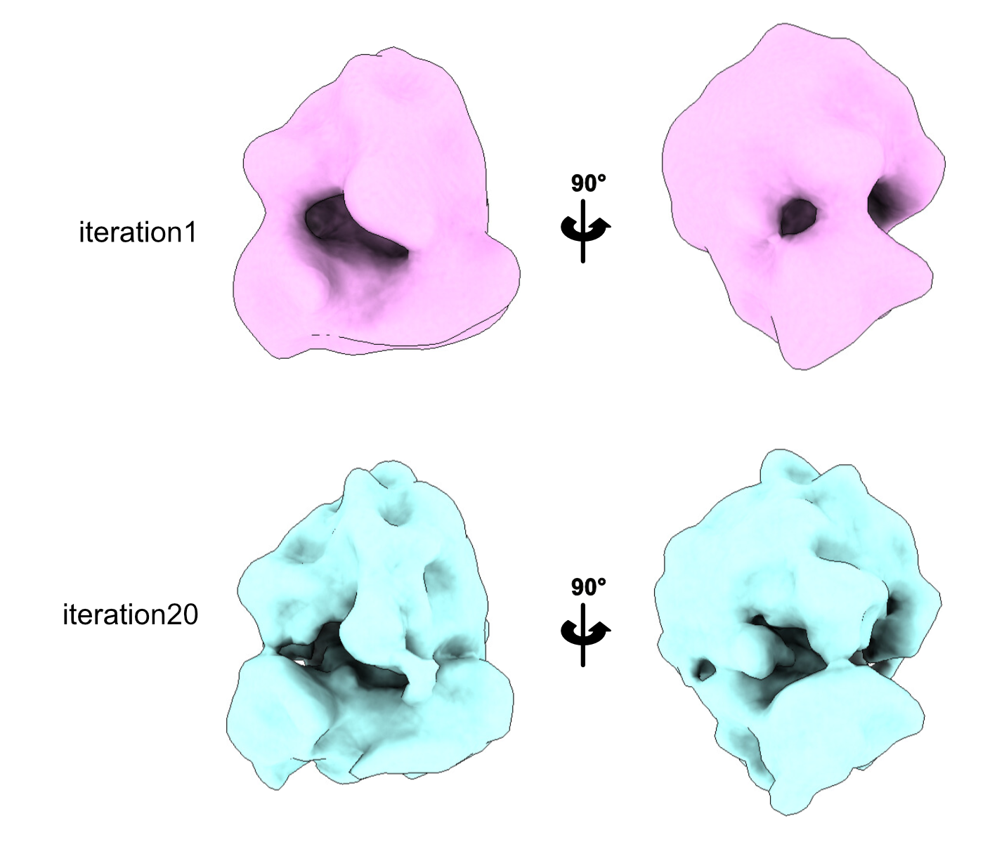
You can see that at iteration 1, our ribosome is very smooth; you can only distinguish the large and small subunit. At iteration 20, we start seeing domains.

3D classification without alignment

Your particles should now be all aligned, more or less the same way. The next step would be to run classification without alignment, but this might be different for you.

Let’s again launch a Class3D job.

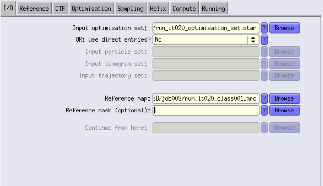
I/O Tab

• Input images STAR file: Use the *_data.star file generated by the previous 3Dclass job. E.g., if you liked iteration 9, you have to use run_it009_data.star as input.
• Reference map: Use the run_it009_data.mrc file created by the 3Dclass job.

Reference Tab

• Initial low-pass filter: You can now set the low-pass filter slightly above the resolution given by the iteration you reached in the 3DClass with 1 class. In that case, we were at 21 Å, so let’s set it to 25 Å.

Optimisation Tab

• Number of classes: This now depends on the heterogeneity you expect and the number of particles you have. Start maybe with 6 classes, but this parameter should be changed and tested.
• T parameter: This is a parameter that you will have to play with. Usually, launching multiple jobs with different T values is smart (e.g 0.5, 1, 2 and 4).

Sampling Tab

• Perform alignment: Set to No this time

Compute Tab

• Turn off GPU acceleration

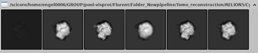
To check the progress of the classification, can check each iteration in the ~/Class3D/job00X and open the volumes run_it00x_class001.mrc in ChimeraX or IMOD. You can also follow it in RELION. Go to File > Display (or Alt+D) and open Class3D > job00X > run_it000_model.star.

This would show you a 2D slice of all your classes, which can sometime be helpful to judge about the quality of the classes.

Like this, for example:

By left clicking on the class you are selecting it. If you right-click you have different options, and statistics available.

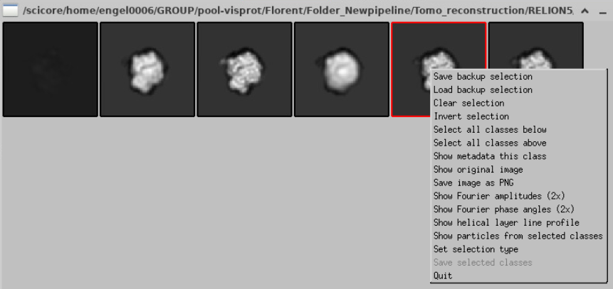
You can click on Show metadata this class

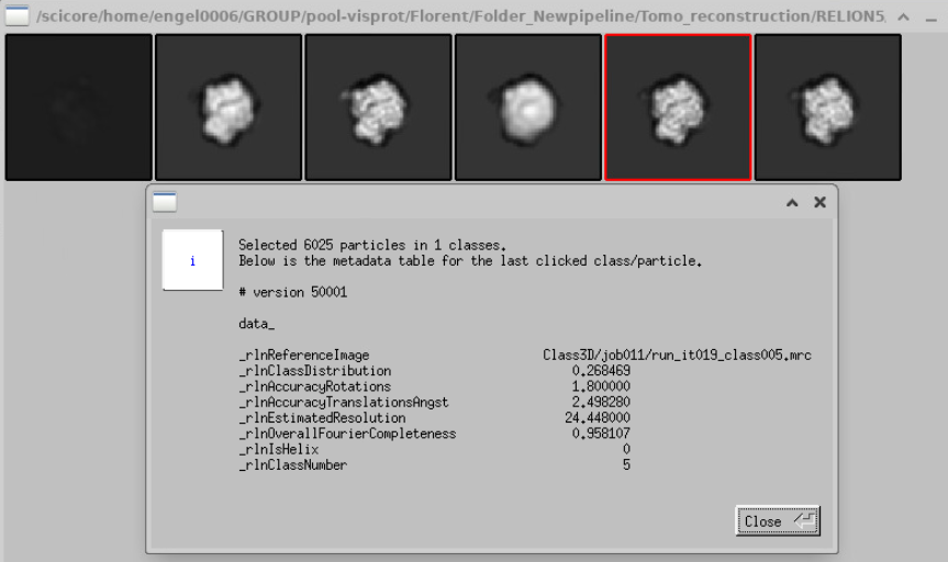
And you can see how many particles are in that class, the estimated resolution, etc … Of course, you can also open all these classes in ChimeraX to see how they look:

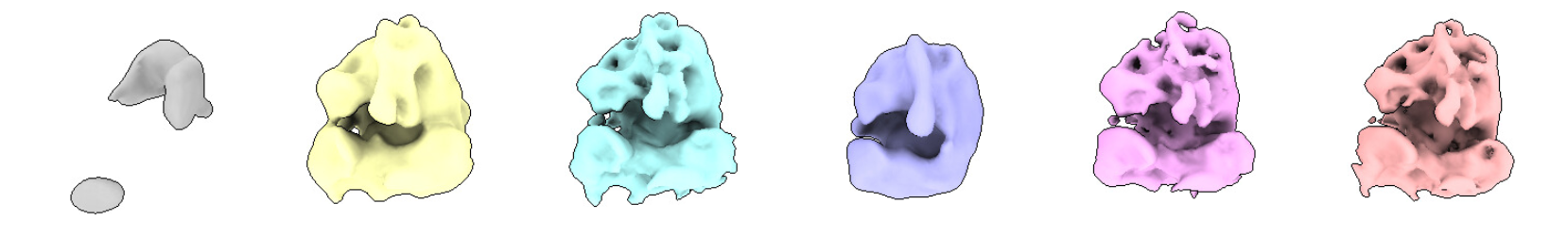
You can see that class 1 is an empty or “trash” class. Classes 2, 3, 5, and 6 are quite similar, with class 2 being less resolved. Class 4 is bad.

Same as before, you can also monitor the classification in RELION, using the commands described previously.

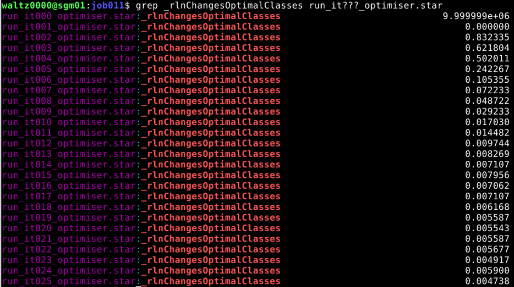
Here we are tracking how much the particles are changing classes. You can see that after iteration 19, not much is happening anymore. So we will use this.

Select good classes

Assuming your classification worked and you want to select good classes (es), and only proceed with these.

Let’s launch a Subset selection job.

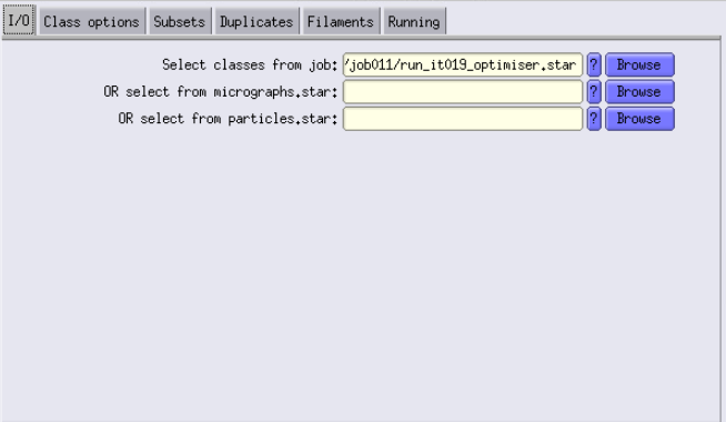
I/O Tab

For the Input images STAR file, take the particles file that was created by the Class3D job, at the iteration that you want. For example, if you liked iteration 24, you have to use Class3D/job00X/run_it019_optimiser.star as input.

All the other tabs should be set to No

Running Tab

Don’t submit it to the queue, run it locally!

Press Run!

The Relion display GUI pops up, press Display! This will show you a 2D slice of all your classes. It’s similar to the Display tab.

To select the one(s) you want, left click on it/them. Then press right click, and do Save selected classes. Also, BEFORE SAVING, you can right-click and do Show metadata this class, and it will show you the total number of particles you are selecting.

Close the windows, it RELION should tell Saved Select/job00X/particles.star with XXXXX selected particles.

Here’s an example of selected classes:

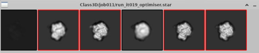
You can see that we selected classes 2, 3, 5 and 6.

In that case, we could have also discarded class 2, that have less defined features, but we decided to be generous with the particle selection because we know that some will improve later. We will do a second round of classification without alignment at bin2, where we will be more selective.

Creating a mask

Something that we haven’t done yet is create a mask.

​In single-particle analysis (SPA) and subtomogram averaging (STA), masks are essential tools used to enhance the accuracy and resolution of reconstructions. They serve several key purposes:​

Focus Alignment and Classification: Masks isolate specific regions of interest within a particle, such as a flexible domain or a particular subunit. By focusing computational efforts on these areas, masks improve alignment precision and enable targeted classification, which is crucial for resolving structural heterogeneity.​

Noise Reduction: Applying masks helps exclude extraneous noise from surrounding areas, such as solvent regions or neighbouring particles. This exclusion enhances the signal-to-noise ratio, leading to clearer and more accurate reconstructions.

For the next steps we will use a mask that cover the entire ribosome and ​exclude the solvent, to make sure that alignment is only focused on the ribosome.

To do so, let’s launch a Mask creation job.

I/O Tab

You will use a map of the ribosome that you working with. The best is to use, for example, class 3 or 5 of iteration 19 from our last 3D classification job.

Mask Tab

These are the parameters that are going to be used to create the mask. The important ones are “Lowpass filter”, “Initial binarisation threshold” and “Extend binary map this many pixels”

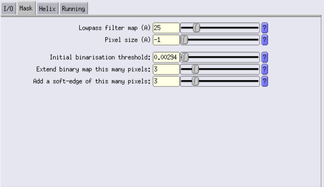
For the Lowpass parameter, let’s use 25, which is slightly lower than the resolution we are at.

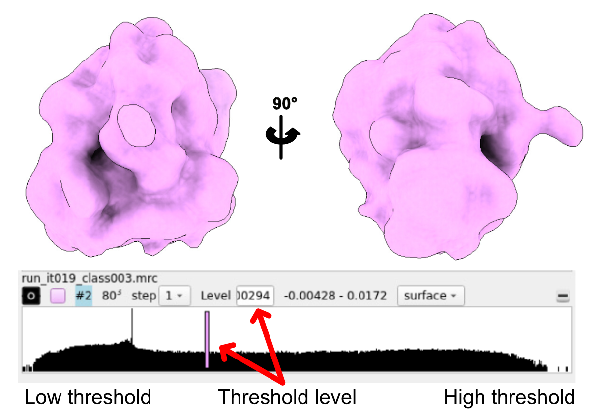
For the Initial binarisation threshold, you will have to open your input map in ChimeraX, and decide of the threshold you want to use. We recommend choosing a rather low threshold, to be sure to have all the features of ribosome are visible, even the low resolution ones.

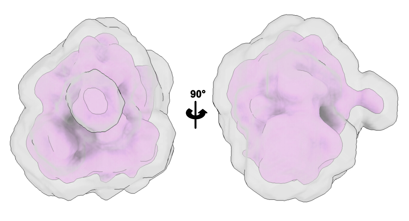
We will then extend by 3 pixels, to make sure that the mask is not going to cut through our volume.

You can then create the mask, and check how it looks (always check!)

3D Refinement

Let’s now do a proper 3D alignment using 3D Refinement.

The 3D auto-refinement job aligns particle images to iteratively reconstruct a high-resolution 3D map of a macromolecule. To ensure accuracy and prevent overfitting, the dataset is split into two independent half-sets. Each half is refined separately, and their similarity is assessed using the gold-standard Fourier Shell Correlation (FSC). This is the specific part which was not done 3D classification with 1 class. This approach ensures that only genuine structural features are enhanced during refinement.

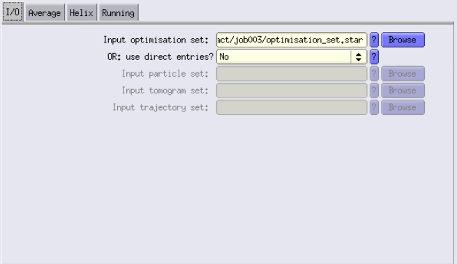
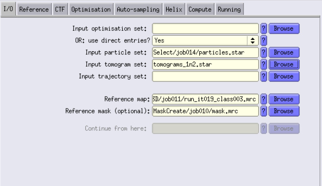
I/O Tab

• This time, we can not use the Input optimisation set, because we created a subset of particles. We have to use direct entries. Set it to Yes
• For the Input particle set, use the output of the Select job
• For the Input tomogram set, I use the tomogram.star that contains all the tomograms (from gain ref 1 and 2). You can easily create it by just copying and pasting the list of tomo within these files.
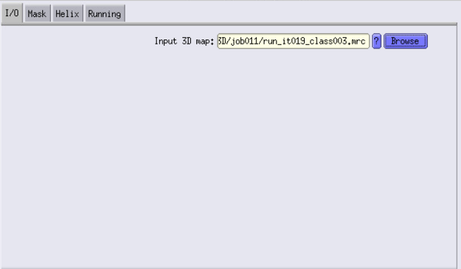
• Reference map: Here I use the run_it019_class003.mrc from the 3D classification job that I used to create the mask.
• Reference mask: Use the mask.mrc we just made before.

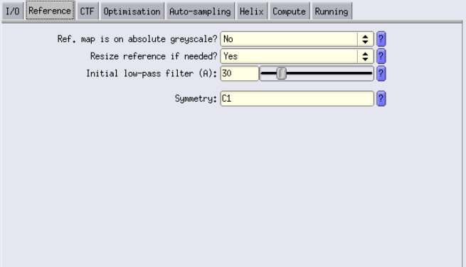
Reference Tab

• Initial low-pass filter: Let’s go with 30 Å.

CTF Tab

• Same as 3D classification

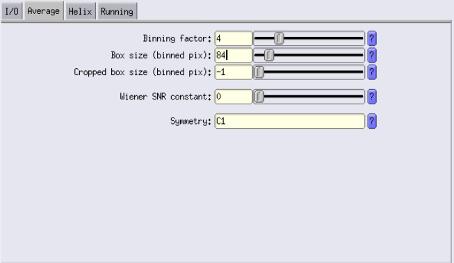
Optimisation Tab

• Mask Diameter: Is the same as in 3D classification, 570. Note: this mask is different from the mask we just created; it’s a spherical mask, automatically created by RELION.
• Use solvent-flattened FSCs: In the case of STA, this has proven particularly useful, set it to YES

Auto-sampling Tab

• We again are going to perform only local searches. To enable this, set the “initial angular sampling” and “local searches from auto-sampling” fields to the same values.

Compute Tab

• Configure settings as shown (same as for 3D classification)

Adapt the running parameters, and press Run!

The job will run and stop automatically until it converges. In our case, it ran for 10 iterations, and reached 15.67 Å resolution

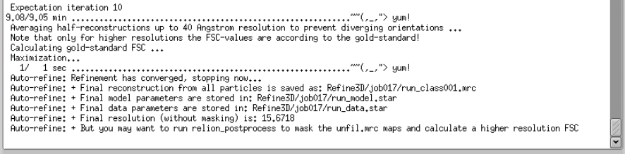
This is very close to Nyquist bin4. Let’s run a Post-processing job to check what the actual resolution is.

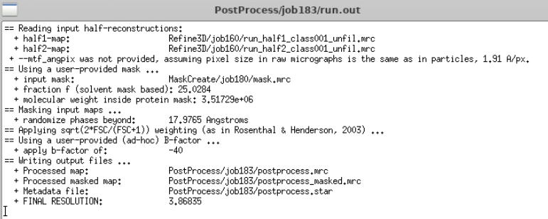
Post-processing

​In RELION, the Post-processing job refines the final 3D map after auto-refinement by performing the following tasks.

1. Mask Application: Applies a user-defined solvent mask to the half-maps to exclude noise from the solvent region, which can otherwise lower the Fourier Shell Correlation (FSC) curve and underestimate resolution.
2. FSC Calculation: Computes the gold-standard FSC between the masked half-maps to provide an accurate resolution estimate.
3. B-factor Sharpening: Automatically estimates and applies a B-factor to sharpen the map, enhancing high-resolution features. ​

The output includes a sharpened map and a PDF summarising the FSC curves and Guinier plots, facilitating assessment of map quality and resolution.

I/O Tab

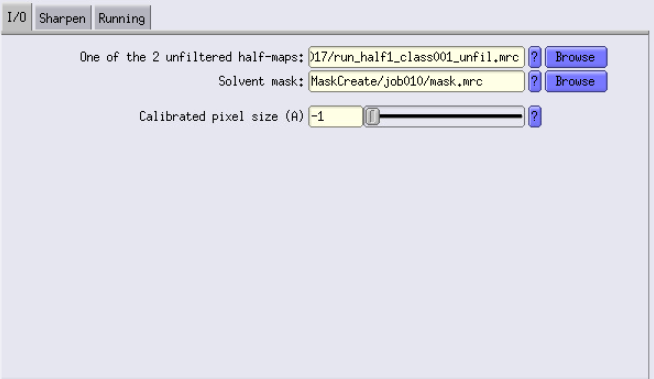
• Unfiltered half-maps: This is the output of the 3D auto-refine job.
• Solvent mask: Use the mask created earlier.
• There is also an option to change the pixel size here if you think the pixel size is slightly off.

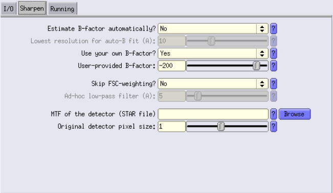
Sharpen Tab

• Estimate B-factor automatically: At this resolution, set it to No. This feature doesn’t work well unless you are already at around 6 Å.
• Use your own B-factor: Set it to Yes and use -200.

Run the job (it’s fast):

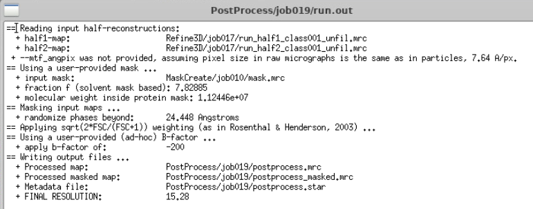
We are at Nyquist bin4!

Check your output, postprocess_masked.star in ChimeraX, it should look sharper than what you had before, and at high threshold, you should already see some rRNA helices.

More classification or going to High-resolution?

After 3D auto-refine you should have reached bin4 Nyquist, which corresponds to the physical limit of the dataset at this particular binning. At bin4, pixel size is 7.64 Å, Nyquist is twice this value, 15.28 Å.

You can further classify your particles using 3D class without (or with) alignment and try to pull out e.g membrane-bound ribosomes or different translation states.

But before doing that we would first recommend running a first round of CTF Refine and Polishing to greatly improve the quality of your particles/average.

CTF and alignment refinement cycle

In the tomo branch of RELION5, CTF refinement and Bayesian polishing are used to improve the quality of subtomogram averages by correcting for optical and motion-related errors.

CTF refinement refines per-particle defocus and optical aberrations using a high-resolution bin1 reference. Bayesian polishing corrects for particle motion across the tilt series, basically realigning your tilt series at the particle level and for the entire tilt series.

Iterative refinement cycle

1. Generate bin1 reference and mask
2. Run CTF refinement
3. Reconstruct at bin1 and post-process
4. Run Bayesian polishing
5. Reconstruct again and post-process
6. Re-extract your particles (at bin 2 or 1)
7. Refine particles
8. Repeat for further improvements

This cycle is typically run after the first classification and refinement, and repeated to progressively improve resolution. Each iteration should result in better maps, both visually and by FSC resolution.

Before starting, you have to do the following:

• Generate a bin1 reference: run a Reconstruct job from your last refinement (at bin4) but resconstruct with bin1 and appropriate box size (4 times your bin4 box size). Use the output of Refine3D as input here.

• Generate a bin1 mask: from the bin1 Reconstruct job generate a bin1 mask
• Post-process: using the bin1 Reconstruct and the generated bin1 mask (the resolution should already be higher than what you obtained that bin4).

In our case, the Post-process already gave 9.55 Å (aka subnanometer resolution 😎).

Run CTF refinement

You should play with different parameters at this step.

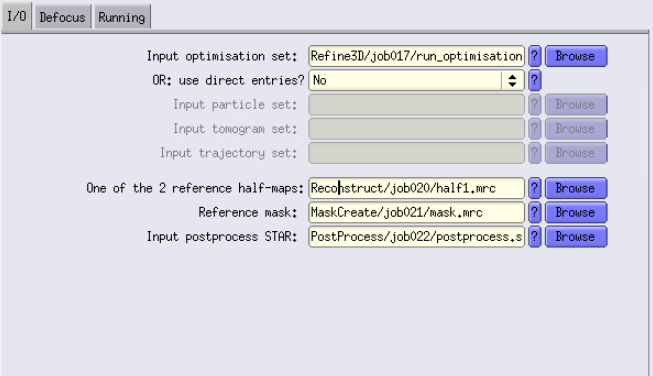
I/O Tab

For the input, use the output of Refine3D. For the half-maps, use the ones generated from the bin1 Recontruct job, use the bin1 mask and the post-process that you ran.

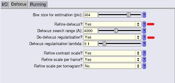
Defocus Tab

This is where you should play with the parameters. Usually, we just change Refine defocus and Do defocus regularization (marked in red). For the Box size for estimation, it is recommended to use a larger box size than your actual box size (again, check the magic box sizes)

Run the jobs with the different parameters, and then for each of them run a Reconstruct job with the same parameters that you used as the step before and run post-process (all with the same bin1 mask you used initially!) and compare resolution. You should also check if, visually, in ChimeraX, the map looks better. At this step resolution should have improved slightly. In our case, we went to 8.48 Å, a whole angstrom gained!

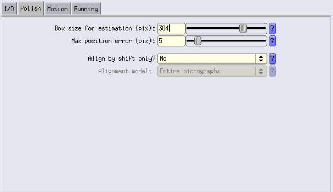
Run Bayesian polishing

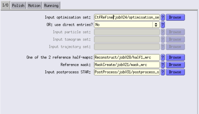
I/O Tab

Use as input the best Ctf Refine job and its respective Reconstruct and Post-Process jobs. Use the same mask you use originally.

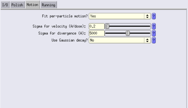
Polish and Motion Tabs

Similarly to Ctf Refine, use a larger box size for estimation than your actual box size (use the same value), and play with the different parameters. Here you can try deactivating Fit per-particle motion, even though it should always be better when turned on.

Again, for each of the Polish jobs, run Reconstruct with the same parameters that you used as the step before and run post-process (all with the same mask!) and compare resolution. At this step resolution should have improved again. In our case, we went to 5.65 Å!

Summary of the first cycle we did (Post-processed value)
Bin4 Refine3D = 15.28 Å (Nyquist bin4)
Reconstruct Bin1 before = 9.55 Å
After CTF Refine = 8.48 Å
After Polish = 5.65 Å

You can see we already reached 5.6 Å, which is already quite cool.

What to do next?

At this step, you should already be quite satisfied, but you can try to push the resolution further. To do this, you should try to align and classify your particles at bin2.

You can re-extract subtomos at bin2 from your best Polish job, then generate a bin2 reference. From there, launch a 3D Refine at bin2 (you should reach Nyquist bin2 ). You can then run a 3D classification job to remove particles that do not positively contribute to resolution (I would not recommend classifying at bin1, except if you are classifying for a feature only visible at bin1).

From there, select the best particles or your sub-state of interest.

Then run another cycle of CTF Refine + Polish. This should improve the resolution even further.

Finally, you can re-extract subtomos at bin1 and run a 3D refinement at bin1, and then again run another cycle of CTF Refine + Polish.

Using 20506 particles from 33 tomograms, here’s the result after 3 cycles of Polishing/refinement, focused on the large subunit of the ribosome. It’s at Nyquist bin1.

Here’s the final map obtained, with some details. We can see RNA base separation, kinda cool!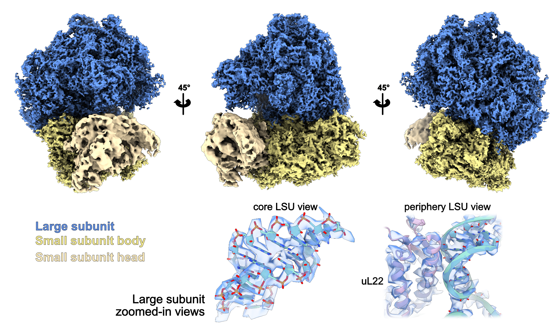

Congrats! You might also be at bin1 Nyquist, the true physical limit of the dataset … or is it? Since this dataset was acquired in EER format, you can in theory go past Nyquist!

Additionally, each Bayesian polishing step generates a new ‘tomograms.star’ that you can use to create polished tomograms on which Template Matching should perform better, because they are better aligned.

Time to start over!

That’s it! Thanks for following this tutorial.